Modeling the Induced Polarization (IP) of Shaly Sands

Vinegar-Waxman Approach

GEOPHYSICS, VOL. 49, NO. 8 (AUGUST 1984); P. 1267-1287

Harold Vinegar & Monroe Waxman (Waxman-Smits Equation) made the incorrect assumption that "the quadrature conductivity Cq was directly proportional to Qv" (a pore volume weighted cation exchange capacity (CEC)).

Mistake #1

Assuming that Cq was proportional to Qv

They chose a “quadrature” formation factor based on the empirical observation that adding a factor of porosity " f” resulted in a better fit to the data

Needed an "unexplainable" (refer below) factor of "f" to match their measurements

This discovery should have been a clue that their original assumption might be wrong. It was not until Mark Rosen's pioneering research into the RF dielectric behavior of shaly sands that the truth was discovered. He too was initially misled by their IP work. The RF dielectric behavior for a small subset of their original IP samples (all having similar porosities) could be successfully described by Qv. However, polarization taking place in the rock is a total volume weighted phenomenon, not a pore volume weighted one. Mark Rosen invented a new petrophysical parameter Qbv that has been shown to correctly quantify the polarization due to clay in shaly sands (refer to Qbv webpage). Harold and Monroe's Qv term in their IP equation reduces to Qbv for the case of m*=2 as shown below:

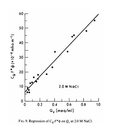
The essence of Harold and Monroe's rather long paper with its almost overwhelming detail (seemingly giving more authority to their model than warranted) is simply this -- a simple linear least squares fit of their measurements to their proposed equation 

as shown in Figure 9 of their paper below:

Based on his RF dielectric research, Mark Rosen (in 1985) proposed a much simpler equation using his newly created petrophysical parameter Qbv:

The results of fitting these two different equations to the IP measurements are shown below:

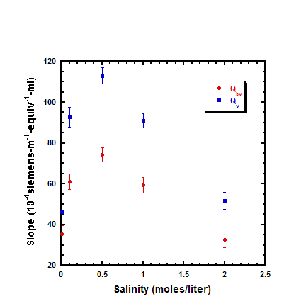
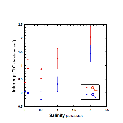
The significant difference between these two equations is the resulting intercepts. The Qv intercept initially goes negative then positive (no possible physical explanation). The Qbv intercept is always positive and increases with salinity indicating that it probably arises from an interfacial polarization component. Harold and Monroe made another mistake by dropping the intercept term, biasing their equation toward very shaly sands as shown by comparing their measurements of two different shaly samples with the various possible equations (Qv without intercept, Qv including intercept, Qbv)

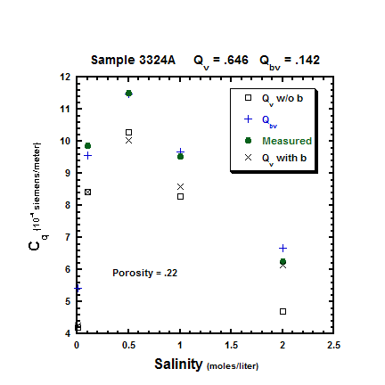
The less shaly sample (3477) demonstrates how significant the error in dropping the intercept term can be. Harold and Monroe were not justified in neglecting this term.

Mistake #2

Dropped the intercept biasing their equation toward very shaly sands

The two graphs above do demonstrate that the Qv equation including the intercept and the Qbv equation give very similar results (they should as shown ealier). The question might arise as to which formulation should be used. The obvious answer is the Qbv equation since it is consistent with higher frequency dielectric measurements (i.e., Qbv correctly quantifies the polarization due to clay from low frequencies (IP) to high frequencies (RF)). Occam's Razor (made famous in the movie Contact) can also be invoked -- the simpler explanation should prevail.

NOTE: The information on this page was shared with both Harold Vinegar and Monroe Waxman -- neither had any corrections or comments. The fact that they were both aware of this analysis back in 1985 (internal Shell research report which was explicitly shared with them), raises serious questions about why they continued to present their model to the technical community (presentations and patents) when they knew it was wrong.